Data analysis using a pipeline

This notebook gives an example of analysing data using the pre-implemented BasicPlus analysis pipeline of the qpcr.Pipes sub-module. It makes use of the provided example data in the Example Data directory.

Experimental background

The corresponding experimental setup was as follows: Levels of Nonsense-mediated mRNA decay (NMD) sensitive (nmd) and insensitive (prot) transcript isoforms of HNRNPL and SRSF11 were measured by qPCR. As normalisers both 28S rRNA and Actin transcript levels were measured. The replicates are biological triplicates and technical douplicates. All measurements from the same qPCR sample were merged into hexaplicates (6 replicates). This was done in two separate HeLa cell lines (one with a specific gene knockout (KO), and one without (WT)), which were both treated to a plasmid-mediated rescue (+) or not (-), leading to four experimental conditions:

cell line \ condition	rescue	no rescue
knockout	KO+	KO-
wildtype	WT+	WT-

Simple Analysis

In this example we will perform the same basic Delta-Delta Ct analysis, we did in the manual tutorial from 1_manual_tutorial.ipynb. However, this time weill be using the pre-implemented BasicPlus pipeline of the qpcr.Pipes sub-module to make our life easier.

# import what we need
from qpcr.Pipes import BasicPlus
from qpcr.Plotters import PreviewResults

Step 1 - Setting up the Pipeline

1.1 Setting up the BasicPlus pipeline

Conveniently, we do not have to define our own qpcr.SampleReader and qpcr.Analyser etc. anymore as the pipeline will handle this already. When using the pipelines our only concern is linking the data and specifying the experimental setup. Additionally, we can link qpcr.Plotters objects such as the PreviewResults figure class to inspect our results later on.

# setup the pipeline
pipeline = BasicPlus()

# (yes, that's it already...)

If we wanted to save the results to a specific location (which we normally would like to do) we can set a specific location to save to using the save_to method.

pipeline.save_to("./Example Results")

1.2 Setting up the data

The pipeline is designed to work either with a list of filepaths or with directory paths that contain the datafiles (if normalisers and sample assays are stored separately). Since we already generated filepath lists in the previous tutorial we will simply re-use these here.

# get our datafiles
normaliser_files = [
                        "./Example Data/28S.csv",
                        "./Example Data/actin.csv"
                ]

sample_files = [
                    "./Example Data/HNRNPL_nmd.csv",
                    "./Example Data/HNRNPL_prot.csv",
                    "./Example Data/SRSF11_nmd.csv",
                    "./Example Data/SRSF11_prot.csv",
            ]

# define our experimental parameters
reps = 6
group_names = ["WT-", "WT+", "KO-", "KO+"]

1.3 Setting up the Preview for later

Since we want to generate a preview of our results, we can just get the qpcr.Results object and use its dedicated preview method to get our preview. Alternatively, we could manually setup one (or multiple different) qpcr.Plotter objects and link them directly to the pipeline. The pipeline will then make a figure with each of them automatically for us.

Here set up a qpcr.Plotters.PreviewResults instance (which is what the qpcr.Results.preview method does as well) that we can link to the pipeline.

# setup our preview
preview = PreviewResults()

# and link our preview to the pipeline
pipeline.add_plotters(preview)

Step 2 - Feed our data to the pipeline

Next we feed our pipeline with our experimental data.

# first we add the experimental setup
pipeline.replicates(reps)
pipeline.names(group_names)

# now we add the datafiles
pipeline.add_assays(sample_files)
pipeline.add_normalisers(normaliser_files)

Step 3 - Running everything

3.1 Hitting the run() button 🕹

Now that we are all set up, we are ready to go. The only thing to do now is to run the pipeline by calling the run() method.

# run the pipeline
pipeline.run()

Step 4 - Inspecting the results

4.1 Getting our results

In order to get our results we can, again, use the get() method. For pipelines the get() method can return either pandas DataFrames with the individual replicate values or summary statistics, or the underlying qpcr.Results object. Check out the documentation for more details.

# get our results as summary statistics (that's the default return format)
summary_stats = pipeline.get()

# and inspect
summary_stats

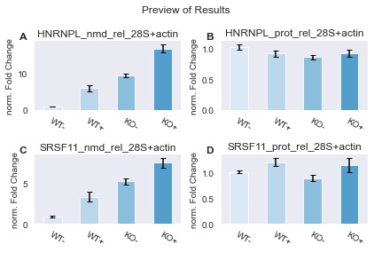
	group	group_name	assay	n	mean	stdev	median	IQR_(0.25, 0.75)	CI_0.95
0	0	WT-	HNRNPL_nmd_rel_28S+actin	6	1.050056	0.029452	1.050267	0.038511	[1.0161980755868047, 1.0839147340669306]
4	1	WT+	HNRNPL_nmd_rel_28S+actin	6	6.052860	0.890336	6.366251	1.516539	[5.029330209330722, 7.076390063511062]
8	2	KO-	HNRNPL_nmd_rel_28S+actin	6	9.566500	0.513593	9.614924	0.734027	[8.976073861884581, 10.156926829088912]
12	3	KO+	HNRNPL_nmd_rel_28S+actin	6	16.940332	1.126687	16.964906	1.096016	[15.645093462670095, 18.235569627233723]
1	0	WT-	HNRNPL_prot_rel_28S+actin	6	1.025239	0.040091	1.006244	0.028966	[0.9791503057437683, 1.0713284193830188]
5	1	WT+	HNRNPL_prot_rel_28S+actin	6	0.913758	0.050860	0.917271	0.042987	[0.8552897342904139, 0.9722270525874591]
9	2	KO-	HNRNPL_prot_rel_28S+actin	6	0.856658	0.029906	0.862768	0.028070	[0.8222776478939225, 0.891038325780611]
13	3	KO+	HNRNPL_prot_rel_28S+actin	6	0.925665	0.057855	0.931949	0.073664	[0.859154910656904, 0.9921743211393722]
2	0	WT-	SRSF11_nmd_rel_28S+actin	6	0.885403	0.102865	0.857620	0.172183	[0.7671489539924317, 1.0036564706179987]
6	1	WT+	SRSF11_nmd_rel_28S+actin	6	3.374373	0.638138	3.644576	0.813222	[2.6407697994029142, 4.107976488500923]
10	2	KO-	SRSF11_nmd_rel_28S+actin	6	5.286670	0.347279	5.284115	0.661335	[4.8874376127697445, 5.685901849372261]
14	3	KO+	SRSF11_nmd_rel_28S+actin	6	7.604066	0.580553	7.770230	0.771464	[6.936662966465831, 8.271469831244389]
3	0	WT-	SRSF11_prot_rel_28S+actin	6	1.009713	0.031999	0.997147	0.053565	[0.9729276202797885, 1.0464986201225999]
7	1	WT+	SRSF11_prot_rel_28S+actin	6	1.197983	0.076915	1.190168	0.126247	[1.1095617597701253, 1.2864044289031957]
11	2	KO-	SRSF11_prot_rel_28S+actin	6	0.887404	0.060800	0.894811	0.102612	[0.8175079293860618, 0.9572992427668053]
15	3	KO+	SRSF11_prot_rel_28S+actin	6	1.136573	0.139244	1.096490	0.174390	[0.9764976866134043, 1.2966473268737058]

At this point we have reached the end of this tutorial. You are now able to use the BasicPlus pipeline to analyse your data. The Basic pipeline works just the same, except that it does not support the linking of a Plotters.

"""
Here is just again our entire workflow with all the code we just wrote:
"""
# get our datafiles
normaliser_files = [
                        "./Example Data/28S.csv",
                        "./Example Data/actin.csv"
                ]

sample_files = [
                    "./Example Data/HNRNPL_nmd.csv",
                    "./Example Data/HNRNPL_prot.csv",
                    "./Example Data/SRSF11_nmd.csv",
                    "./Example Data/SRSF11_prot.csv",
            ]

# define our experimental parameters
reps = 6
group_names = ["WT-", "WT+", "KO-", "KO+"]

# setting up the pipeline
pipeline = BasicPlus()
pipeline.save_to("./Example Results")

pipeline.replicates(reps)
pipeline.names(group_names)

# setup our preview
preview = PreviewResults(mode = "static")
pipeline.add_plotters(preview)

# feed in our data
pipeline.add_assays(sample_files)
pipeline.add_normalisers(normaliser_files)

# run the pipeline
pipeline.run()
# and at this point the results are already saved :-)