Decorating datafiles

This notebook gives an example how to decorate your irregular or Big Table datafiles. It makes use of the provided example data in the Example Data directory.

1 - Decorating an “irregular” datafile

An “irregular” datafile stores it’s assays in separate tables that are either above one another or next to one another. To decorate the assays we have to add the decorators @qpcr:assay and @qpcr:normaliser wihtin the cell immediately above the assay header.

Note

Your assay headers must be either all in the same column or row!

See how in the file below we have decorated the assay for 28S as a normaliser and the one below for HNRNPL as an assay :

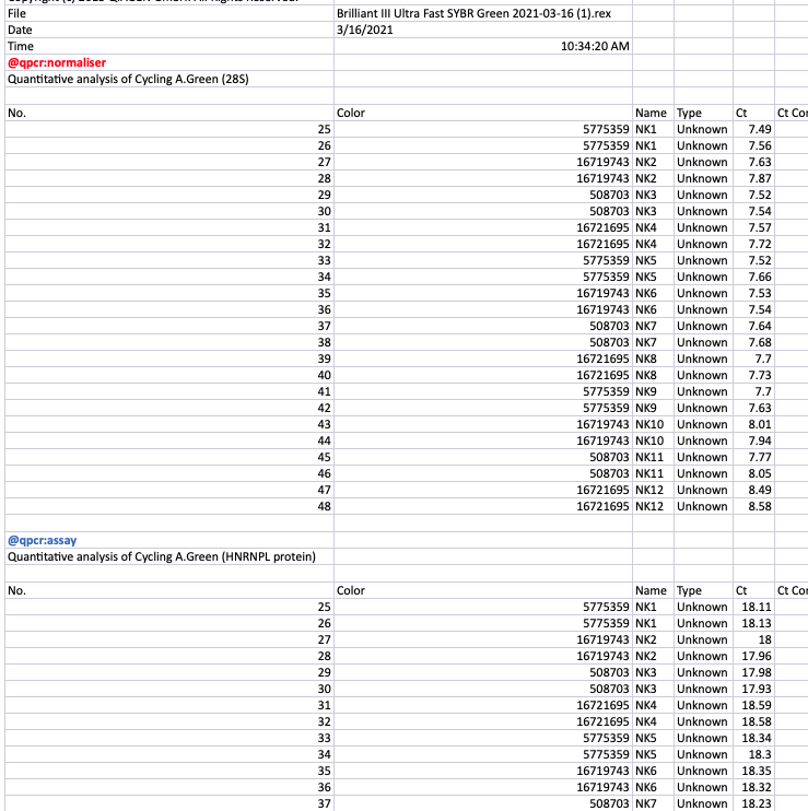
This exact scheme we can now follow for any assay within our datafile. Note, this also works on multi-sheet excel files. However, when working with Excel, you will likely have to add a single tick ' in front of the decorator to escapt it’s being interpreted as a function.

Note

If you decorate your data, and specify that it’s decorated when reading with one of the qpcr.Readers any and all non-decorated assays will be ignored!

The same approach naturally also works for horizontal irregular datafiles (this will require the option transpose = True when working with the qpcr.Readers or the transpose() method when working directly with the qpcr.Parsers).

The decorated file below is from Hernandez (2018). It and all following files below were obtained from Zenodo for the purpose of this tutorial.

2 - Decorating a Big Table datafile

Big Table files store all their assays wihtin a single datatable, which is either “vertical” or “horizontal”.

The @qpcr decorator column

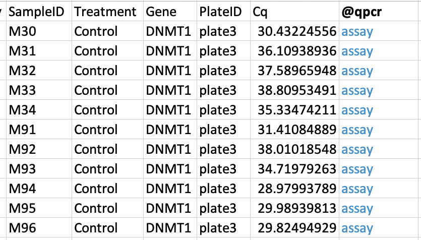
Both kinds of tables allow “decoration” by adding a @qpcr column that stores the values assay or normaliser. The purpose of the column is probably self-evident at this point.

The file below is a vertical Big Table file from Holmann et al. (2015). Notice the @qpcr column at the very right?

The @qpcr:group decorator

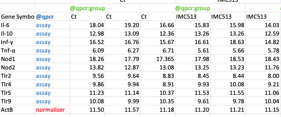
For “horizontal” Big Tables, we require some more decoration to read. Because “horizontal” Big Tables store the replicate Ct values in side-by-side columns qpcr requires the decorator @qpcr:group to be in the cell immediately above the first replicate Ct value column of each group.

The decorated file below is from Garcia-Gonzalez et al. (2020). Notice, how a @qpcr:group decorator is placed above the first columns of the Ct and IMC513 groups. Also, there is a @qpcr column denoting assays and normalisers. A little disclaimer at this point, Garcia-Gonzalez et al. did not actually include the ActinB values, they were added for this overview. Why are they not included? In fact, the values in the table are already delta-delta-Ct values! However, for the purpose of this tutorial their data arrangement is the only thing of importance.

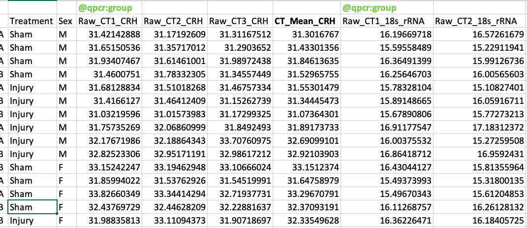
Why does qpcr require the group-decorators?

Well, the reason is best explained by looking at a file from Howe et al. (2020). Their data includes triplicates for assays CRH and 18s rRNA. However, they also include columns with the replicate means as well. Now, such additional data columns within the data, no matter where they are located within the Big Table, actually make it impossible to just “split” the table by rows and be done. Also, notice how the column names of the triplicate Ct values are not identical?

Hence, qpcr can also not rely on identically named columns to find the data. To solve this problem without forcing the user to overly meddle with their data arrangement, qpcr opted to just rely on some additional decorators. The replicate values must be specified manually in this setting, of course. Therefore, a little more manual user effort is required to read such a datafile, but the decorator approach allows for an arbitrary amount of additional data to be stored alongside the raw Ct values, and is thus also appropriate for re-visiting and -analysing already exisiting data easily.

With this we have reached the end of this tutorial. Adding decorators to your data is really easy. How we can then work with the decorated files using the qpcr.Readers and qpcr.Parsers has already been introduced in the previous two tutorials. You now know a very powerful way to speed up your analyses. Congrats!